1. Aggregate Demand - Macroeconomics Tutor

Part 1: Introduction to Aggregate Demand

This video is the first in a set of four explaining the Hicks-Hansel model of Keynes' theory of Aggregate Demand, specifically the IS-LM interpretation. This model is very important to short run macroeconomics and attempts to explain shifts in the aggregate demand curve and what determines national income for any price level

These topics are usually taught in an intermediate Macroeconomics class, and these videos are intended as a visual aid to further your understanding of the models.

This video reviews the components of aggregate demand, income, the consumption function. taxes, finding equilibrium in this short run model, and the factors affecting the slope and position of the aggregate demand curve. The second video covers the IS curve, regarding the goods market, the third video covers the LM curve regarding the money market and the final video puts the two together to find equilibrium in both markets

Components

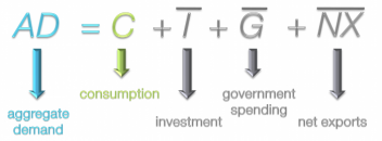
We begin our discussion of Aggregate Demand by looking at its components and their symbols. You will likely be familiar with the concept of Aggregate Demand, the total demand for all finished goods in the economy. It is usually broken down into the demand for the following factors:

C for Consumption, I for Investment, G for Government Spending and NX for Net Exports. Some textbooks break it down into exports and imports but net exports is simply exports minus imports.

Initially we will only consider changes in consumption, making investment, government spending and net exports exogenous to our model which we designate by putting a horizontal bar over top of them.

Consumption Function

To begin we're going to look at how consumption is related to income. We're going to break down consumption into its separate components. Beginning with autonomous consumption. This is the base level of consumption. In this model, consumption cannot fall below autonomous consumption, regardless of what people are making as income. Next we have disposable income. This is the "after tax" income. Although "disposable income" is commonly used as the money you have remaining after you've paid your rent and bills, that's now what it means in economic terms. Disposable income is multiplied by the coefficient c, the "marginal propensity to consume". This tells us how much consumption increases for every $1 increase in income. The MPC coefficient can be between zero and one.

Consumption Function Graph

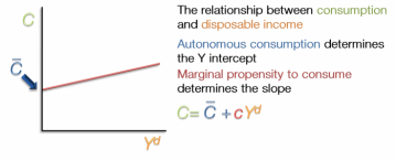
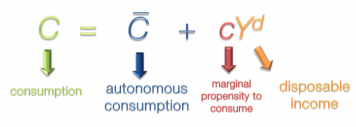
Graphically, the consumption function displays the relationship between consumption and disposable income. Consumption, the dependent variable, is on the Y-axis. Disposable income, the independent variable, is on the X-axis. The level of autonomous consumption determines the Y-intercept. As you recall, this is the level of consumption when disposable income is zero. Marginal propensity to consume determines the slope of this curve. As disposable income increases from left to right it is modified by the MPC. A high MPC of 0.9 would lead to a steep curve. A lower MPC would mean a more gradual slope.

Income

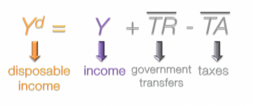
Now we're going to take a closer look at disposable income. This is an aggregate measure of all the income paid to households plus government transfers (such as welfare of social security) minus income taxes. As it's presented here, government transfers and taxes do not change relative to our dependent variable, income. Again, this is shown by the horizontal bar above the two exogenous variables.

Generally income taxes are some percentage of income. Although it's not that simple in practice, in this model we're going to think of taxes as flat rate, denoted by the lower case t. The coefficient could be any number between zero, meaning no tax, and one, meaning all income would be paid in taxes. This is then multiplied by income.

Now that our disposable income has taxes incorporated into it, we're going to plug it back into the consumption function.

Taxes

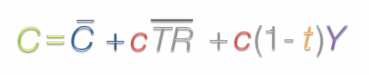
Here is the consumption function as previously shown. Disposable income is now replaced with tax-rate formula. Some simple algebraic factoring will clean up this formula. The terms with Income in them are grouped together, leaving the transfer payments to be multiplied by MPC. To simplify the bottom term, Y is taken out the bracket, leaving one minus taxes, all multiplied by MPC. Putting it all together we have the updated consumption function that includes income tax. Consumption = autonomous consumption + transfer payments + MPC x (1- taxes ) x income.

Aggregate Demand Equation

Next incorporate this updated consumption function into the aggregate demand equation. The first step is to separate the factors into exogenous, and endogenous. Exogenous demand is represented by A-bar. Investment, government spending and net exports are exogenous because they aren't affected by national income in this model, so their value won't change when income changes. These factors will be grouped at the bottom under A-bar. When we substitute the consumption function in for C we can see that there are some exogenous variables, such as exogenous consumption and transfer payments. These can be grouped down below with the other external factors. We can bring two groups together with the simplified A-bar to represent all of the exogenous factors and the c(1-t)Y representing the determining factors.

Equilibrium Output

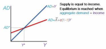
In this model, aggregate supply is equal to income at any point in time. Therefore, supply=demand when aggregate demand= income. When we have aggregate demand on the y axis and income on the x-axis, equilibrium is reached at any point on the 45° angle, where the values for both axis are equal.

The aggregate demand curve starts out on Y-axis at a value equal to the exogenous demand (A bar) and then continues upward with increasing levels of income. Equilibrium occurs when the two lines intersect, this indicates the equilibrium income and equilibrium level of aggregate demand.

Change in MPC

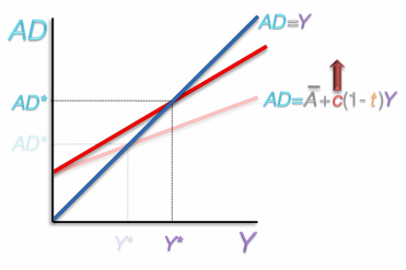
Moving forward we are going to see how equilibrium changes in reaction to a change in the Marginal Propensity to Consume. If a country becomes more inclined to spend their disposable income, their MPC is larger. An increase in the marginal propensity to consume creates a steeper aggregate demand curve. The point of origin is the same, but steeper line crosses the equilibrium line at a higher point. This results in larger equilibrium values for aggregate demand and national income.

Change in Tax Rate

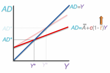
If there is a change tax rate, say from 30% to 50%, the slope will be more gradual, resulting in lower equilibrium levels of aggregate demand and national income.

Change in Exogenous Demand

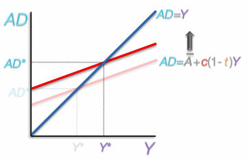
A change in Exogenous Demand would result from a change in any of the following, autonomous consumption, transfer payments, investment, government spending, or net exports. If there was an increase in any of these components, the entire aggregate demand curve would shift up. This leads to higher equilibrium values for aggregate demand and national income. Note that the slope remains unchanged in this scenario.

This concludes the introduction on Aggregate Demand. Please watch the second video, which explains how to find equilibrium in the goods market