Goods Market
This section covers the finding simultaneous equilibrium in the goods market and the money market by combining the IS and LM curves. This leads to a method for deriving the Aggregate Demand curve. This model is also used to anticipate the economy's response to fiscal and monetary policy.
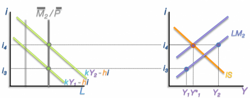
This slide displays the goods and services market on the top right hand side. The money market is on the left.
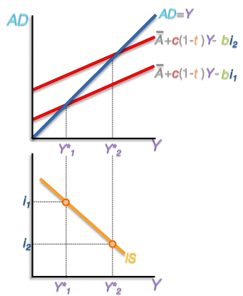
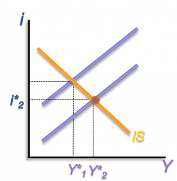
First, in the goods market, the horizontal line is the equilibrium condition and the aggregate demand equation extends upward. The equilibrium interest rate and level of income are extended down to derive the IS curve. The higher interest rate results in a higher equilibrium income. Connecting these points creates the IS Curve.
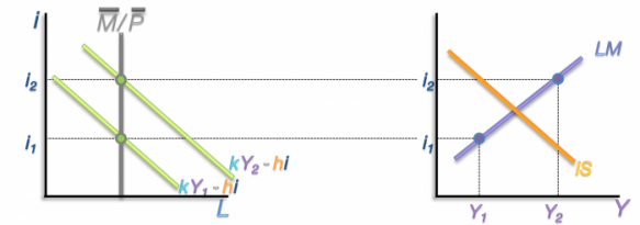
In the money market, on the left, the real money supply is the grey vertical line. When the demand for money curve crosses it the equilibrium interest rate is found. For a higher level of national income (Y2), the equilibrium interest rate is higher, these points create the LM curve.
The intersection of the IS and LM curves denotes the equilibrium level of interest and income that will have both markets in simultaneous equilibrium.
This slide displays the goods and services market on the top right hand side. The money market is on the left.
First, in the goods market, the horizontal line is the equilibrium condition and the aggregate demand equation extends upward. The equilibrium interest rate and level of income are extended down to derive the IS curve. The higher interest rate results in a higher equilibrium income. Connecting these points creates the IS Curve.
In the money market, on the left, the real money supply is the grey vertical line. When the demand for money curve crosses it the equilibrium interest rate is found. For a higher level of national income (Y2), the equilibrium interest rate is higher, these points create the LM curve.
The intersection of the IS and LM curves denotes the equilibrium level of interest and income that will have both markets in simultaneous equilibrium.
Money Market
In the money market, on the left, the real money supply is the grey vertical line. When the demand for money curve crosses it the equilibrium interest rate is found. For a higher level of national income (Y2), the equilibrium interest rate is higher, these points create the LM curve.
Simultaneous Equilibrium
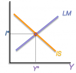
The intersection of the IS and LM curves denotes the equilibrium level of interest and income that will have both markets in simultaneous equilibrium.
Deriving the Aggregate Demand Curve
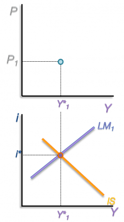
From this information we can derive the aggregate demand curve in the Price/Income graph on the top right. This is done by finding the IS-LM equilibrium for different price levels. Price levels are in the real money supply equation that is represented by the grey vertical bar. By drawing LM curves for different price levels, we can produce enough points in the P/Y space to derive the aggregate demand curve.
The LM curve is drawn for the first price level, producing the first point at the intersection of P1 and the resulting equilibrium level of national income.
The LM curve is drawn for the first price level, producing the first point at the intersection of P1 and the resulting equilibrium level of national income.
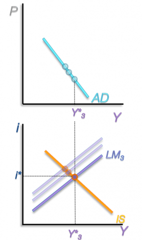
A reduction the price level increases the real money supply because people can buy more with the money they have. The lower price level shifts the money supply line outward. This causes the LM curve to shift down and the equilibrium income (Y2) to be further to the right. Where this line intersects with P2, the second point of the Aggregate demand curve is drawn. This process could be repeated again to produce an even higher level of equilibrium with lower prices. By connecting these points the downward sloping demand curve is formed.
Monetary Policy
Now for the reactions of the markets to a change in monetary policy. If the central bank increases the money supply (M) the real money supply line shifts outward and the LM curve shifts outward accordingly.
Here is the LM curve being formed for M1, a low supply of money. This forms the first point of equilibrium at i1 and Y1.
When the central bank increases the money supply to M2 the LM curve shifts down.
Here is the LM curve being formed for M1, a low supply of money. This forms the first point of equilibrium at i1 and Y1.
When the central bank increases the money supply to M2 the LM curve shifts down.
The immediate result is that the interest rate drops from its original equilibrium to the intersection of Y1 and the lower LM curve. This is based on the assumption that the money markets adjust quickly. At this point the money market is in balance because the point is on the LM curve, but the interest rate is too low for the goods market to be in equilibrium. At this position there is an excessive demand for goods so output and income start to increase. The Money market adjusts quickly to the increased income: an increase in income increases the demand for money and in turn increases the interest rate. This plays out as the point of equilibrium moves up the LM curve until it reaches the IS curve. At this point the interest rate and Income stabilize and the economy reaches equilibrium. So the end result of the policy of increasing the money supply lower interest rates and a higher level of national income.
Fiscal Policy
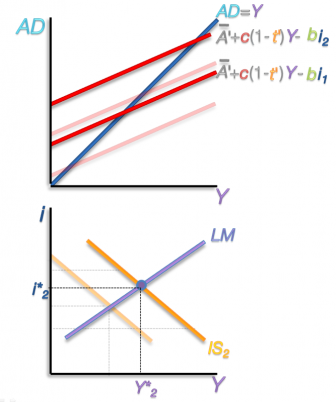
Fiscal policy takes the form of government spending. The two red aggregate demand functions contain exogenous demand, of which government spending is a factor. Here the IS curve is derived using the first value of exogenous demand. Equilibrium income and interest rate are found.
By increasing government spending the red aggregate demand curves are shifted upward. The resulting IS2 is shifted outward. The money market quickly responds and a new point of equilibrium is reached at i2 and Y2. So by increasing government spending, the equilibrium level of national income has risen and the interest rate has also risen.
By increasing government spending the red aggregate demand curves are shifted upward. The resulting IS2 is shifted outward. The money market quickly responds and a new point of equilibrium is reached at i2 and Y2. So by increasing government spending, the equilibrium level of national income has risen and the interest rate has also risen.
