Part 3: LM Curve
The LM curve is used to determined equilibrium in the money market. The L stands for liquidity and M for Money. The video covers the demand for money, the supply of money, the LM curve, the factors affecting its slope and position and finally the algebraic formula for the curve.
Demand for Money
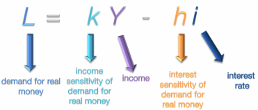
Demand for real money is represented by the letter 'L'. Real money is adjusted for inflation, so this indicates the actual purchasing power of money. The amount of demand depends on income, because that determines the amount people have to spend and it depends on the interest rate because money can be put to better use if it is invested. As the minus sign indicates, the higher the interest rate, the more inclined people are to invest their money rather than having it available to spend.
These two variables are moderated by sensitivity coefficients: the income sensitivity of demand for real money and the interest sensitivity of demand for real money. Both of these have a value greater than zero.
These two variables are moderated by sensitivity coefficients: the income sensitivity of demand for real money and the interest sensitivity of demand for real money. Both of these have a value greater than zero.
Demand for Money Graph
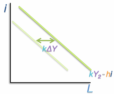
Now we're going to examine this relationship graphically. Interest rate, the independent variable, goes on the Y-axis because its going to be relating to the LM graph, which as interest rate on the same axis. Demand for money, the dependent variable, goes on the X-axis. As the interest rate decreases, the demand for money increases, which gives us the downward sloping demand for money curve.
An increase in the national income results in an upward and outward shift of the demand for money curve. The amount of shift depends on the increase in income as well as the income sensitivity of demand for money.
An increase in the national income results in an upward and outward shift of the demand for money curve. The amount of shift depends on the increase in income as well as the income sensitivity of demand for money.
Increase in Interest Sensitivity of Demand for Money
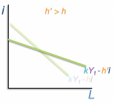
An increase in the interest sensitivity for real money reduces the slope of the demand for money curve. The original h value is low because a large drop in interest rate is required to increase the demand for money.
h' is higher, meaning the interest sensitivity is higher. The slope is less steep which means a relatively small decrease in interest rate causes a large increase in the demand for money.
h' is higher, meaning the interest sensitivity is higher. The slope is less steep which means a relatively small decrease in interest rate causes a large increase in the demand for money.
Money Supply
Now that we've covered the demand for money, we're going to introduce the supply of real money. This is composed of the nominal money supply, the number value of all the cash balances in a country. In this model the amount of money is set by the central bank and therefore exogenous. This value is divided by price level, the correction for inflation. Since this model is applied to the very short run, inflation is not a factor so the price level is exogenous. This calculation produces the real money supply.
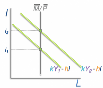
Represented graphically, the money supply is a vertical line. In the very short run it is fixed. This graph shows two demand for money curves for different levels on national income. The intersection of the demand for money curves and the money supply line indicate the equilibrium rates of interest, i1 and i2.
Represented graphically, the money supply is a vertical line. In the very short run it is fixed. This graph shows two demand for money curves for different levels on national income. The intersection of the demand for money curves and the money supply line indicate the equilibrium rates of interest, i1 and i2.
LM Curve
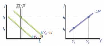
We're ready for the LM curve. On the left we have the money demand/money supply graph. The LM curve will be graphed in the interest, income space on the left. The vertical money supply line is already showing. Here is the demand for money curve for Y1. The point at which it crosses the money supply line produces the first equilibrium rate of interest, i1. This line is extended to the LM space and creates our first point as it intersects with Y1. This is repeated for a higher level of national income, Y2. This produces the second equilibrium rate of interest, i2. We extend this line across to the LM space and it intersects with Y2. These two sampled points are all we need to draw the LM curve. It denotes the levels of national income and interest rates that allow the money market to be in equilibrium.
Slope of the LM Curve
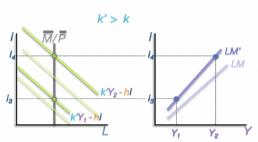
Now we're going to examine the determinants of the LM curve's slope. Here we have the original LM curve. We're going to increase the income sensitivity of demand for real money, k. When we graph the new demand for money curves on the left they have shifted upward. Because k' is a coefficient of Y, the upward shift for Y2 will be even more pronounced. When the new equilibrium interest rates i3 and i4 are extended over to the LM space we can see that the slope of the LM curve has increased.
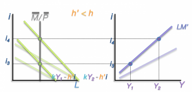
In this example the initial demand for money curves are relatively flat. We're going to decrease the interest sensitivity of demand for real money. The curves produced with the lower h' indicate that it would take a relatively large decrease in interest rate to produce a dramatic increase in the demand for money. When the lines are drawn for both our sample income levels we see that the resulting LM curve's slope has increased.
***Correction: In the video I read this as income sensitivity but it should be interest sensitivity***
***Correction: In the video I read this as income sensitivity but it should be interest sensitivity***
Position of LM
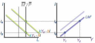
As for the position of the LM curve, this is determined by the real money supply. An increase shifts the money supply line outward. The resulting equilibrium interest rates are lower. This results in a downward shift of the LM curve.
Algebraic Relationship
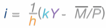
Now that we've gone through the relationship graphically, we're going to examine this equilibrium condition algebraically. Here is the demand for real balances formula. Equilibrium is reached when supply equals demand so we will substitute real money supply in for L. We want to solve this equation for 'i' because it is the dependent variable in the LM curve. We bring 'h i' over to the left side of the equation and move the money supply to the right side. We divide both sides by h', the interest sensitivity of demand for money. It cancels out on the left side and stays on the right side. And here is the formula for the LM curve. This will give you the equilibrium interest rates for different levels of national income, Y.
Slope of LM Curve
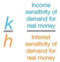
The slope of the LM curve is the coefficient of Y, k over h, or the income sensitivity of demand for real money over the interest sensitivity of demand for real money. This ratio is important for monetary policy.
That concludes the video on the LM curve. It covered the demand for money, the supply of money, the LM curve, the factors affecting its slope and position and then the formula behind it. Please watch the next video regarding the interaction of IS and LM curves and the policy implications of the model.
That concludes the video on the LM curve. It covered the demand for money, the supply of money, the LM curve, the factors affecting its slope and position and then the formula behind it. Please watch the next video regarding the interaction of IS and LM curves and the policy implications of the model.
